Code
# Exercise 3
a <- 100In this exercise we will get acquainted with R. A convenient way to work with R is with RStudio, as RStudio adds many features and convenient accessibility options to the plain R you have obtained from http://r-project.org. Most of these features go beyond the scope of this course, but as you will develop your R skillset, you might run into the need for RStudio at a later moment. Best to get to know RStudio now.
If you have no experience with R, you will learn the most from following this document. If you have some experience with R already, I suggest you try solving the questions without looking at the answers/walkthrough. You can then refer to the solutions at any time, if needed.
If you have any questions or if you feel that some code should be elaborated, feel free to ask me via e-mail or ask the workgroup instructor.
We start with the very basics and will move towards more advanced operations in R. First we will get acquainted with the language and the environment we work in.
RStudioThe following window will appear. 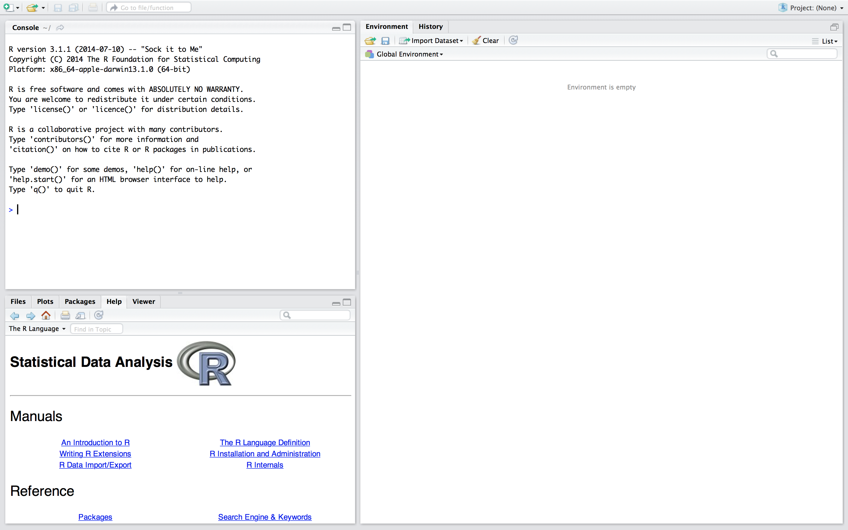
RStudio is divided in 3 panes, namely the console, the environment/history pane and the pane where we can access our files, plots, the help files, make packages and view our data objects. You can change the order of the panes to your liking through RStudio’s preferences. I did, that is why your pane layout might differ from the layout in the above screenshot.
If we open an R-script (i.e. a file that contains R code), a fourth pane opens.
R-script.In the top left you will find  . Click it and select
 R-script.
A new pane opens, and we can start typing our code. It is preferable to work from an R-script instead of directly working in the console for at least the following reasons (there are many more).
RStudio caches files even if they are not saved.R-script and data, others are able to exactly reproduce your work. Reproducibility is becoming increasingly more important, and this is where RStudio excells.R-script# Exercise 3
a <- 100The # tells R that everything that follows in that specific line is not to be considered as code. In other words, you can use # to comment in your own R-scripts. I used # here to elaborate that the following line is the code from exercise 3.
The line a <- 100 assigns the value 100 to object a. When you run your code, it will be saved. The value 100 and the letter a are chosen to illustrate assigning in R. You might as well assign 123 to banana if you like. Really, anything goes.
Your code is executed and now appears in the console. If you type a in the console, R will return the assigned value. Try it. 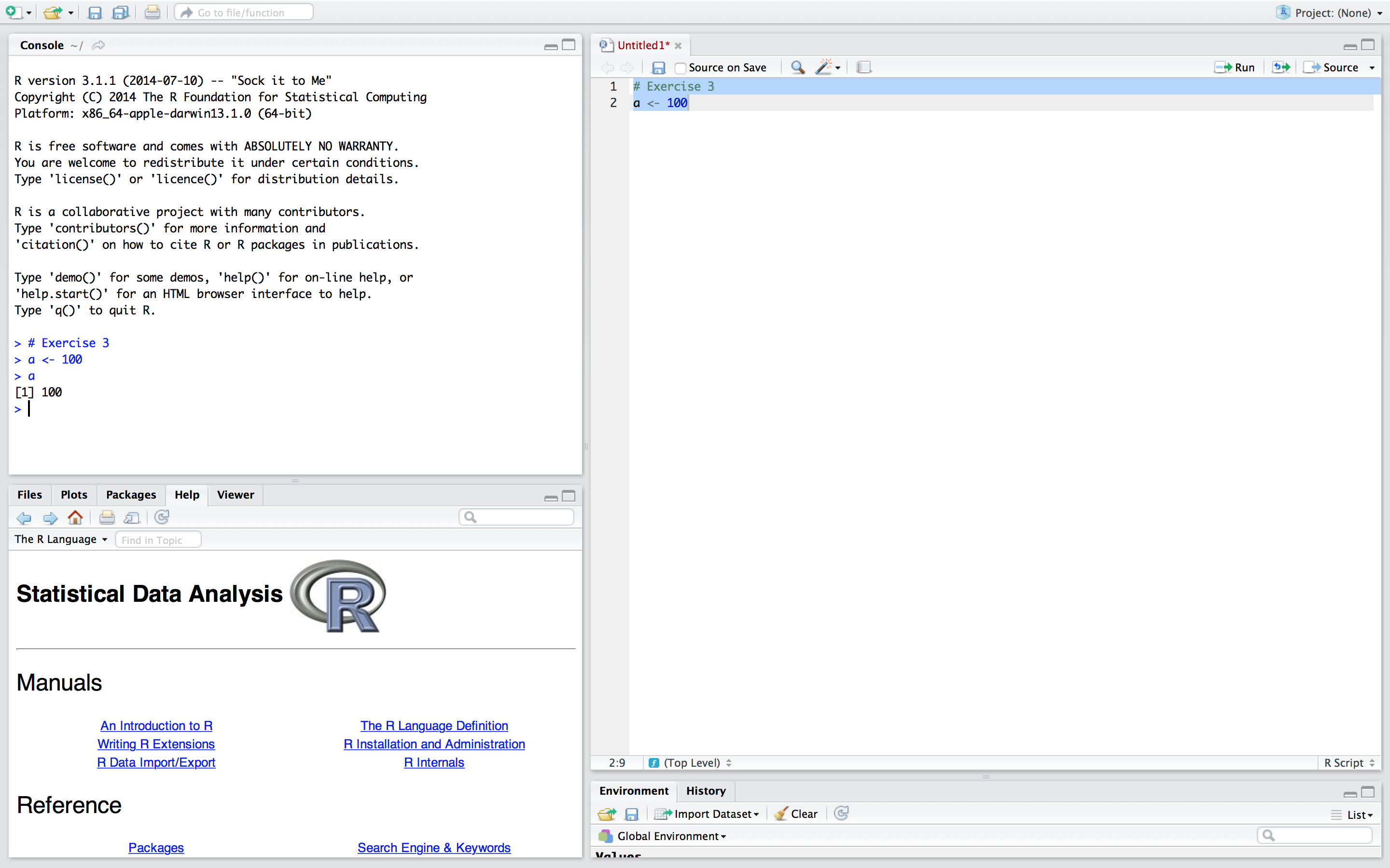
The shortcut Ctrl-Enter or Cmd-Enter is your friend: it runs the current selection, or, if nothing is selected, the current line. if Ctrl-Enter or Cmd-Enter yields no result, you probably have selected the console pane. You can switch to the code pane by moving the mouse cursor and clicking on the desired line in the code pane, or through Ctrl-1 (Windows/Linux/Mac). Alternatively, you can move to the console through Ctrl-2 (Windows/Linux/Mac).
This is how you enter and run code in R by using RStudio.
Practical_1.R in a folder named PracticalsYou can use the standard Ctrl-s (Windows/Linux) or Cmd-s (Mac) or click on the icon  in the code pane.
Your document is now saved. We saved it in a separate folder so that we are able to create a project out of our practicals.
 in the top-right corner of
 RStudioSelect New Project, click Existing Directory and navigate to the folder where you have just saved your code. When all is done, click on Create Project
You will notice in the files pane that a file Practicals.RProj has been created
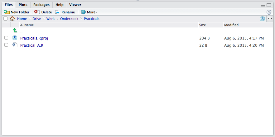
The possibility to categorize your work in projects is one of the benefits of using RStudio. Within a project, everything is relative to the .Rproj file. This means that if you share the folder with someone else, this someone only has to open the .Rproj file to be able to access and run all code and documents involved with this project. Again, when considering reproducability of research, working in projects is a huge advantage.
R-script notebook.R. You can find notebook.R here.
html file. Click on the  icon and select
 html as the notebook output format. The benefit of using html as an output format lies in the dimensional properties of a web-page. Especially when dealing with long code-files, large output from analyses or many graphs, exporting your file as html is much more convenient. You can simply scroll down or up to see the ‘rest’, instead of having to flip through pages back and forth to compare code, graphs or output.
html file you have created. The notebook feature in R-Studio is very convenient; it runs and converts any R-code to a readable file where code and output are visible. There is, however, an even better format to integrate R-code with text into a single document: Markdown!
rmarkdown and quartoWhat is R Markdown? from RStudio, Inc. on Vimeo.
See also this rmarkdown cheat sheet.
In a nutshell, rmarkdown provides a way to create nice documents containing r code and its output.
In 2022, RStudio launched Quarto. Quarto is the natural extension to rmarkdown. The main differences are that Quarto contains some nice extra features and supports languages other than R, as Python or Julia.
For beginners, we recommend using the more modern Quarto. That is what we will cover in the workshop. However, you are likely to still encounter rmarkdown docs and references in the wild, so it is good to know it exists. Besides,rmarkdown will still be maintained, so it is likely that both formats will coexist, at least for a while. You can read more about the differences between Quarto and rmarkdown here. You can read more about Quarto on its website, with very detailed documentation and tutorials
The existence of two very similar tools for the same thing might sound as unnecessarily complicated, but do not worry: rmarkdown and Quarto are very similar. Indeed, most files written in rmarkdown (.rmd extension) can be run in Quarto by simply changing the extension from .rmd to .qmd. In the few cases files cannot be ran, a few modifications in the code will be sufficient to make it work again.
Quarto.qmd. You can find the notebook quarto.qmd here.
Have a look at the code in the quarto.qmd file and make sure that you understand what is going on. If you do not understand what you are looking at, please ask.
Render to compile the file into a html-document. If necessary, install the required packages. Inspect the html file and compare it to the one you have created from the notebook.R file. In the rest of this course we will need to make exercises and assignments and hand in our materials. The notebook functionality is a convenient way to quickly compile code and discuss it with a teacher and/or your peers. The Quarto functionality in R-Studio is a very polished production device to mark-up high quality documents where text and code are woven together. Please use Quarto to hand in your work and present both the .qmd and .html files whenever you need to hand in exercises or assignments.
#install.packages("tidyverse")End of Practical 1. Play around with R and R-studio if you like. We will be using Quarto documents for the rest of the course.