Practical B

Author

Javier Garcia-Bernardo (adapted from Gerko Vink)

Published

November 27, 2023

Exercises

In this practical exercise we are going to play around with the different types of elements in R.

Click on the Code buttons to see the solutions. Please really try before looking at the solution, and ask the instructor if something is not 100% clear.

First, create a new Quarto document for this practical (File -> New File -> Quarto document)

Exercise 1-4: Vectors and matrices

Make two vectors: one named vec1 with values 1 through 6 and one named vec2 with letters A through F.

Code

vec1 <- c(1, 2, 3, 4, 5, 6)
vec2 <- c("A", "B", "C", "D", "E", "F")

To create a vector we used c(), which stands for ‘concatenation’. It is just a series of numbers or letters.

Create two matrices, one from vec1 and one from vec2. The dimensions for both matrices are 3 rows by 2 columns.

Code

mat1 <- matrix(vec1, nrow = 3, ncol = 2)
mat2 <- matrix(vec2, nrow = 3, ncol = 2)

To create a matrix we used matrix(). For a matrix we need to specify the dimensions (in this case 3 rows and 2 columns) and the input (in this case vec1 or vec2) needs to match these dimensions.

Inspect your vectors and matrices. Are all numerical?

Code

vec1

[1] 1 2 3 4 5 6

Code

vec2

[1] "A" "B" "C" "D" "E" "F"

Code

mat1

     [,1] [,2]
[1,]    1    4
[2,]    2    5
[3,]    3    6

Code

mat2

     [,1] [,2]
[1,] "A"  "D" 
[2,] "B"  "E" 
[3,] "C"  "F"

vec1 and mat1 contain numbers and vec2 and mat2 contain characters.

Make a matrix from both vec1 and vec2 using cbind. Inspect this matrix using is.matrix().

Code

mat3b <- cbind(vec1, vec2)
is.matrix(mat3b)

[1] TRUE

Code

mat3b

     vec1 vec2
[1,] "1"  "A" 
[2,] "2"  "B" 
[3,] "3"  "C" 
[4,] "4"  "D" 
[5,] "5"  "E" 
[6,] "6"  "F"

If one or more elements in the matrix represent characters, all other elements are also converted to characters. A matrix is just for either numeric or character elements. Notice that the second approach (the column bind approach from mat3b) returns a matrix where the column names are already set to the name of the bound objects.

To solve the problem of charactered numbers we can create a dataframe. A dataframe is essentially a matrix that allows for character elements. The use of a dataframe is often preferred over the use of a matrix in R, except for purposes where pure numerical calculations are done, such as in matrix algebra. However, most datasets do contain character information and a dataframe would normally be your preferred choice when working with your own collected datasets in R.

Exercise 5-7: Data frames

Make a dataframe called dat3 where vec1 and vec2 are both columns. Name the columns V1 and V2, respectively. Use function data.frame().

Code

dat3 <- data.frame(V1 = vec1, V2 = vec2)
dat3

Select 1) the third row, 2) the second column and 3) the intersection of these two in the dataframe dat3 that you have created in Question 4.

Code

dat3[3, ] #3rd row

  V1 V2
3  3  C

Code

dat3[, 2] #2nd column

[1] "A" "B" "C" "D" "E" "F"

Code

dat3$V2   #also 2nd column

[1] "A" "B" "C" "D" "E" "F"

Code

dat3[3,2] #intersection

[1] "C"

The [3,2] index is very useful in ‘R’. The first number (before the comma) represents the row and the second number (after the comma) represents the column. For a vector there are no two dimensions and only one dimension can be called. For example, vec1[3] would yield 3. Try it.

Columns can also be called by the $ sign, but only if a name has been assigned. With dataframes assigning names happens automatically.

Note that R automatically reports the values the character column can take. This means that the column is indeed a factor (a categorical variable - as it is supposed to be). A useful function to inspect the structure of a dataframe is str(). Try running it.

Code

str(dat3)

'data.frame':   6 obs. of  2 variables:
 $ V1: num  1 2 3 4 5 6
 $ V2: chr  "A" "B" "C" "D" ...

Inspecting the structure of your data is vital, as you probably have imported your data from some other source. If we, at a later stage, start analyzing our data without the correct measurement level, we may run into problems. One problem that often occurs is that categorical variables (factors in R) are not coded as such.

Imagine that the first variable V1 in our dataframe dat3 is not coded correctly. Instead of digits, it should represent information about cities. Convert the variable to a factor and add the labels Utrecht (corresponding to value 1), New York (value 2), London (3), Singapore (4), Rome (5) and Cape Town (6).

Code

dat3$V1 <- factor(dat3$V1, labels = c("Utrecht", "New York", "London", "Singapore", "Rome", "Capetown"))
dat3

         V1 V2
1   Utrecht  A
2  New York  B
3    London  C
4 Singapore  D
5      Rome  E
6  Capetown  F

Exercise 8-11: Read/explore CSV

Read the file dataset_boys.csv.

First create a folder “data” in your project. Then download it from here and add it to that folder (use Ctrl+S in the browser to download it).

First you need to load the required library to read the CSV (readr). You may need to install it first.

Code

#install.packages(c("readr"),repos = "http://cran.us.r-project.org")
library(readr)

Then you can read the file using the function read_delim() from the readr library

Rows: 748 Columns: 9
── Column specification ────────────────────────────────────────────────────────
Delimiter: ","
chr (3): gen, phb, reg
dbl (6): age, hgt, wgt, bmi, hc, tv

ℹ Use `spec()` to retrieve the full column specification for this data.
ℹ Specify the column types or set `show_col_types = FALSE` to quiet this message.

Code

boys <- readr::read_delim("data/dataset_boys.csv", delim=",")

Code

head(boys)

# A tibble: 6 × 9
    age   hgt   wgt   bmi    hc gen   phb      tv reg  
  <dbl> <dbl> <dbl> <dbl> <dbl> <chr> <chr> <dbl> <chr>
1 0.035  50.1  3.65  14.5  33.7 <NA>  <NA>     NA south
2 0.038  53.5  3.37  11.8  35   <NA>  <NA>     NA south
3 0.057  50    3.14  12.6  35.2 <NA>  <NA>     NA south
4 0.06   54.5  4.27  14.4  36.7 <NA>  <NA>     NA south
5 0.062  57.5  5.03  15.2  37.3 <NA>  <NA>     NA south
6 0.068  55.5  4.66  15.1  37   <NA>  <NA>     NA south

Alternatively, you can import datasets directly from the internet by running and loading the connection

Code

#To update
con <- url("https://javier.science/R/Contents/Material/common_datasets/dataset_boys.csv")

In the above code we store the connection in object con and then load the connectio.

The boys object will be added to your Global Environment. You can now use the boys data by running

Code

boys <- readr::read_delim(con, delim = ",")

Rows: 748 Columns: 9
── Column specification ────────────────────────────────────────────────────────
Delimiter: ","
chr (3): gen, phb, reg
dbl (6): age, hgt, wgt, bmi, hc, tv

ℹ Use `spec()` to retrieve the full column specification for this data.
ℹ Specify the column types or set `show_col_types = FALSE` to quiet this message.

You can explore boys in several ways. In notebooks just write “boys” and run the chunk. You can also use the “Environment” menu to find the data “boys” and double click it. Alternatively write View(boys).

Using View() is preferred for inspecting datasets that are large. View() opens the dataset in a spreadsheet-like window (conform MS Excel, or SPSS). If you View() your own datasets, you can not edit the datasets’ contents.

Find out the dimensions of the boys data set (use the function dim) and inspect the first and final 6 cases in the data set.

To do it numerically, find out what the dimensions of the boys dataset are. Use the function dim()

Code

dim(boys)

[1] 748   9

There are 748 cases on 9 variables. To select the first and last six cases, use

Code

boys[1:6, ]

# A tibble: 6 × 9
    age   hgt   wgt   bmi    hc gen   phb      tv reg  
  <dbl> <dbl> <dbl> <dbl> <dbl> <chr> <chr> <dbl> <chr>
1 0.035  50.1  3.65  14.5  33.7 <NA>  <NA>     NA south
2 0.038  53.5  3.37  11.8  35   <NA>  <NA>     NA south
3 0.057  50    3.14  12.6  35.2 <NA>  <NA>     NA south
4 0.06   54.5  4.27  14.4  36.7 <NA>  <NA>     NA south
5 0.062  57.5  5.03  15.2  37.3 <NA>  <NA>     NA south
6 0.068  55.5  4.66  15.1  37   <NA>  <NA>     NA south

Code

boys[743:748, ]

# A tibble: 6 × 9
    age   hgt   wgt   bmi    hc gen   phb      tv reg  
  <dbl> <dbl> <dbl> <dbl> <dbl> <chr> <chr> <dbl> <chr>
1  20.4  189.  59.8  16.8  55.2 <NA>  <NA>     NA west 
2  20.4  181.  67.2  20.5  56.6 <NA>  <NA>     NA north
3  20.8  189.  88    24.6  NA   <NA>  <NA>     NA west 
4  20.8  194.  75.4  20.1  NA   <NA>  <NA>     NA west 
5  20.8  189   78    21.8  59.9 <NA>  <NA>     NA north
6  21.2  182.  76.5  23.1  NA   <NA>  <NA>     NA east

or, more efficiently:

Code

head(boys)

# A tibble: 6 × 9
    age   hgt   wgt   bmi    hc gen   phb      tv reg  
  <dbl> <dbl> <dbl> <dbl> <dbl> <chr> <chr> <dbl> <chr>
1 0.035  50.1  3.65  14.5  33.7 <NA>  <NA>     NA south
2 0.038  53.5  3.37  11.8  35   <NA>  <NA>     NA south
3 0.057  50    3.14  12.6  35.2 <NA>  <NA>     NA south
4 0.06   54.5  4.27  14.4  36.7 <NA>  <NA>     NA south
5 0.062  57.5  5.03  15.2  37.3 <NA>  <NA>     NA south
6 0.068  55.5  4.66  15.1  37   <NA>  <NA>     NA south

Code

tail(boys)

# A tibble: 6 × 9
    age   hgt   wgt   bmi    hc gen   phb      tv reg  
  <dbl> <dbl> <dbl> <dbl> <dbl> <chr> <chr> <dbl> <chr>
1  20.4  189.  59.8  16.8  55.2 <NA>  <NA>     NA west 
2  20.4  181.  67.2  20.5  56.6 <NA>  <NA>     NA north
3  20.8  189.  88    24.6  NA   <NA>  <NA>     NA west 
4  20.8  194.  75.4  20.1  NA   <NA>  <NA>     NA west 
5  20.8  189   78    21.8  59.9 <NA>  <NA>     NA north
6  21.2  182.  76.5  23.1  NA   <NA>  <NA>     NA east

The functions head() and tail() are very useful functions. For example, from looking at both functions we can observe that the data are very likely sorted based on age.

Inspect the boys dataset with str(). Use one or more functions to find distributional summary information (at least information about the minimum, the maximum, the mean and the median) for all of the variables. Give the standard deviation for age and bmi. Tip: make use of the help (?) and help search (??) functionality in R.

Code

str(boys)

spc_tbl_ [748 × 9] (S3: spec_tbl_df/tbl_df/tbl/data.frame)
 $ age: num [1:748] 0.035 0.038 0.057 0.06 0.062 0.068 0.068 0.071 0.071 0.073 ...
 $ hgt: num [1:748] 50.1 53.5 50 54.5 57.5 55.5 52.5 53 55.1 54.5 ...
 $ wgt: num [1:748] 3.65 3.37 3.14 4.27 5.03 ...
 $ bmi: num [1:748] 14.5 11.8 12.6 14.4 15.2 ...
 $ hc : num [1:748] 33.7 35 35.2 36.7 37.3 37 34.9 35.8 36.8 38 ...
 $ gen: chr [1:748] NA NA NA NA ...
 $ phb: chr [1:748] NA NA NA NA ...
 $ tv : num [1:748] NA NA NA NA NA NA NA NA NA NA ...
 $ reg: chr [1:748] "south" "south" "south" "south" ...
 - attr(*, "spec")=
  .. cols(
  ..   age = col_double(),
  ..   hgt = col_double(),
  ..   wgt = col_double(),
  ..   bmi = col_double(),
  ..   hc = col_double(),
  ..   gen = col_character(),
  ..   phb = col_character(),
  ..   tv = col_double(),
  ..   reg = col_character()
  .. )
 - attr(*, "problems")=<externalptr>

Code

summary(boys) #summary info

      age              hgt              wgt              bmi       
 Min.   : 0.035   Min.   : 50.00   Min.   :  3.14   Min.   :11.77  
 1st Qu.: 1.581   1st Qu.: 84.88   1st Qu.: 11.70   1st Qu.:15.90  
 Median :10.505   Median :147.30   Median : 34.65   Median :17.45  
 Mean   : 9.159   Mean   :132.15   Mean   : 37.15   Mean   :18.07  
 3rd Qu.:15.267   3rd Qu.:175.22   3rd Qu.: 59.58   3rd Qu.:19.53  
 Max.   :21.177   Max.   :198.00   Max.   :117.40   Max.   :31.74  
                  NA's   :20       NA's   :4        NA's   :21     
       hc            gen                phb                  tv       
 Min.   :33.70   Length:748         Length:748         Min.   : 1.00  
 1st Qu.:48.12   Class :character   Class :character   1st Qu.: 4.00  
 Median :53.00   Mode  :character   Mode  :character   Median :12.00  
 Mean   :51.51                                         Mean   :11.89  
 3rd Qu.:56.00                                         3rd Qu.:20.00  
 Max.   :65.00                                         Max.   :25.00  
 NA's   :46                                            NA's   :522    
     reg           
 Length:748        
 Class :character  
 Mode  :character

Code

sd(boys$age) #standard deviation for age

[1] 6.894052

Code

sd(boys$bmi, na.rm = TRUE) #standard deviation for bmi

[1] 3.053421

Note that bmi contains 21 missing values, e.g. by looking at the summary information. Therefor we need to use na.rm = T to calculate the standard deviation on the observed cases only.

Exercise 12-14: Filtering the CSV

Select all boys that are 20 years or older. How many are there?

The logical operators (TRUE vs FALSE) are a very powerful tool in R. For example, we can just select the rows (respondents) in the data that are older than 20 by putting the logical operater within the row index of the dataset:

Code

boys2 <- boys[(boys$age >= 20), ]
nrow(boys2)

[1] 12

or, alternatively (the tidy way),

Code

library(dplyr) #Library to filter


Attaching package: 'dplyr'

The following objects are masked from 'package:stats':

    filter, lag

The following objects are masked from 'package:base':

    intersect, setdiff, setequal, union

Code

boys2 <- dplyr::filter(boys, age >= 20)
nrow(boys2)

[1] 12

Select all boys that are older than 19, but younger than 19.5. How many are there?

Code

boys3 <- boys[(boys$age > 19) & (boys$age < 19.5), ]
nrow(boys3)

[1] 18

or, alternatively,

Code

boys3 <- dplyr::filter(boys, age > 19, age < 19.5)
nrow(boys3)

[1] 18

What is the mean age of boys younger than 15 years of age that do not live in region north?

Code

age_subset <- boys[(boys$age < 15) & (boys$reg != "north"), ]$age
mean(age_subset, na.rm = TRUE)

[1] 6.044461

or, alternatively,

Code

age_subset <- dplyr::filter(boys, (age < 15), (reg != "north"))$age
mean(age_subset, na.rm=TRUE)

[1] 6.044461

The mean age is 6.0444609 years

Exercises 15-17: Visualization

Download the file example_csv.csv from here and add it to your data folder.

Open the file in your text editor to see how it looks. What is the first line?

Read the file and save it with the name “df_events”. You’ll need to use the argument “skip” in the read_delim() function to skip the first line. Make sure it looks fine by printing the head.

Rows: 9 Columns: 2
── Column specification ────────────────────────────────────────────────────────
Delimiter: "\t"
dbl (2): Time, Number

ℹ Use `spec()` to retrieve the full column specification for this data.
ℹ Specify the column types or set `show_col_types = FALSE` to quiet this message.

Code

df_events <- readr::read_delim("data/example_csv.csv", skip = 1)
head(df_events)

Code

head(df_events)

# A tibble: 6 × 2
   Time Number
  <dbl>  <dbl>
1     1      1
2     3      2
3     4      3
4     5      4
5     7      5
6     9      6

Print summary statistics of the dataset

Code

summary(df_events)

      Time            Number     
 Min.   : 1.000   Min.   :1.000  
 1st Qu.: 4.000   1st Qu.:2.000  
 Median : 7.000   Median :3.000  
 Mean   : 6.889   Mean   :3.111  
 3rd Qu.:10.000   3rd Qu.:4.000  
 Max.   :12.000   Max.   :6.000

Plot the time vs the events using the function plot (you’ll learn a better way to plot with Gerko)

Code

plot(df_events$Time, df_events$Number)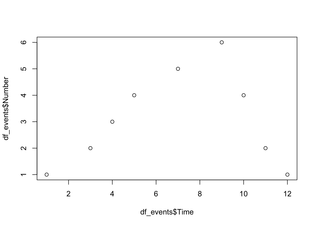

Today we have learned to use R at its basics. This offers tremendous flexibility, but may also be inefficient when our aim is some complex analysis, data operation of data manipulation. Doing advanced operations in basic R may require lots and lots of code. Next you will learn how to use R efficiently.

As you start using R in your own research, you will find yourself in need of packages that are not part of the default R installation. The beauty of R is that its functionality is community-driven. People can add packages to CRAN that other people can use and improve. Chances are that a function and/or package has been already developed for the analysis or operation you plan to carry out. If not, you are of course welcome to fill the gap by submitting your own package.

End of practical